PurpleAir Analysis (January 1-25, 2026)

← Back to Home

Data Acquisition

Data Source

• Platform: PurpleAir Community Sensor Network
• Sensor Model: Plantower PMS5003/PMS6003 optical particle counters
• Data Format: CSV files with 60-minute averages
• Access Method: Direct CSV download from PurpleAir website

Data Characteristics

• Total Sensors: 279 sensors in master sensor list
• Spatial Distribution: Dense urban coverage, with sensors distributed across residential, commercial, and institutional locations
• Temporal Coverage: January 1-25, 2026 (60-minute averages)
• Valid Sensors Processed: 254 sensors with valid data after quality control (91.0% data completeness)
• Sensors Filtered: 25 sensors removed due to outlier values >500 µg/m³ might be due to sensor errors or maintenance issues.

Quality Assurance

• Correction Formula: Applied University of Utah Winter Inversion correction:

  Corrected PM2.5 = (0.778 × Raw_CF1) + 2.65
  

• Outlier Filtering: Removed sensor readings >500 µg/m³ (physically impossible for ambient air, indicating hardware failure)
• Rationale: PurpleAir sensors are optical particle counters that tend to overestimate PM2.5 in high-humidity conditions. The correction formula was derived from co-location studies comparing PurpleAir sensors with EPA FRM monitors under Utah winter conditions.

Advantages

• High spatial density enables detailed neighborhood-level analysis
• Near real-time data availability
• Community-maintained network provides extensive coverage
• Enables spatial interpolation for continuous surface mapping

Limitations

• Requires calibration correction for accuracy
• Variable sensor maintenance quality
• Potential data gaps if sensors go offline
• Different temporal resolution (hourly) compared to EPA daily averages

Technical Methodology

Coordinate System Standardization

• Target CRS: Web Mercator (EPSG:3857)
• Rationale: Standard web mapping projection ensures accurate overlay on basemaps and compatibility with web visualization libraries
• Reprojection: All spatial data (census tracts, sensor locations) converted from WGS84 (EPSG:4326) to EPSG:3857

Data Correction

Correction Formula (University of Utah Winter Inversion):

Corrected PM2.5 = (0.778 × Raw_CF1) + 2.65

Rationale:

• PurpleAir sensors are optical particle counters that tend to overestimate PM2.5 in high-humidity conditions
• Winter inversions in Salt Lake Valley create high-humidity environments
• University of Utah researchers developed this correction formula specifically for Utah winter conditions
• Formula derived from co-location studies comparing PurpleAir sensors with EPA FRM monitors

Application:

• Applied to all raw sensor readings before aggregation
• Correction applied before any spatial analysis or visualization

Quality Assurance

Outlier Detection:

• Physical Impossibility Threshold: PM2.5 > 500 µg/m³
• Rationale: Ambient PM2.5 levels above 500 µg/m³ are physically impossible in urban environments
• Action: Automatically filtered as hardware sensor errors
• Impact: 25 sensors (9.0%) removed from analysis

Visualization Range:

• Color scale capped at 80 µg/m³ to prevent extreme outliers from dominating visualization
• Data preserved for analysis but visually constrained for clarity

Spatial Interpolation

Method: Inverse Distance Weighting (IDW) interpolation

Process:

1. Input Data: Discrete PurpleAir sensor points with corrected PM2.5 values
2. Grid Creation: 200×200 interpolation grid covering study area bounds
3. Interpolation Method: Linear interpolation to create continuous PM2.5 surface
4. Output: Continuous PM2.5 surface as 2D array for heatmap visualization

Spatial Clipping:

• Mask Layer: Census tract boundaries (merged union)
• Purpose: Restrict heatmap visualization to inhabited land areas only
• Result: Clean visualization without pollution data over water bodies, mountains, or uninhabited areas

Data Aggregation

• Temporal Aggregation: Mean PM2.5 per sensor across entire study period (January 1-25, 2026)
• Spatial Representation: Each sensor represented as single point with aggregated value
• Rationale: Enables interpolation between sensors while maintaining individual sensor accuracy

Visualization Approach

• Method: Continuous surface visualization via spatial interpolation
• Color Mapping: OrRd colormap (yellow = low, red = high PM2.5)
• Demographic Context: Side-by-side with census tract choropleth showing population distribution (separate maps for 65+ and 85+)
• Output: High-resolution static maps (300 DPI) and interactive web maps for both age groups

Deliverables

Static Visualizations

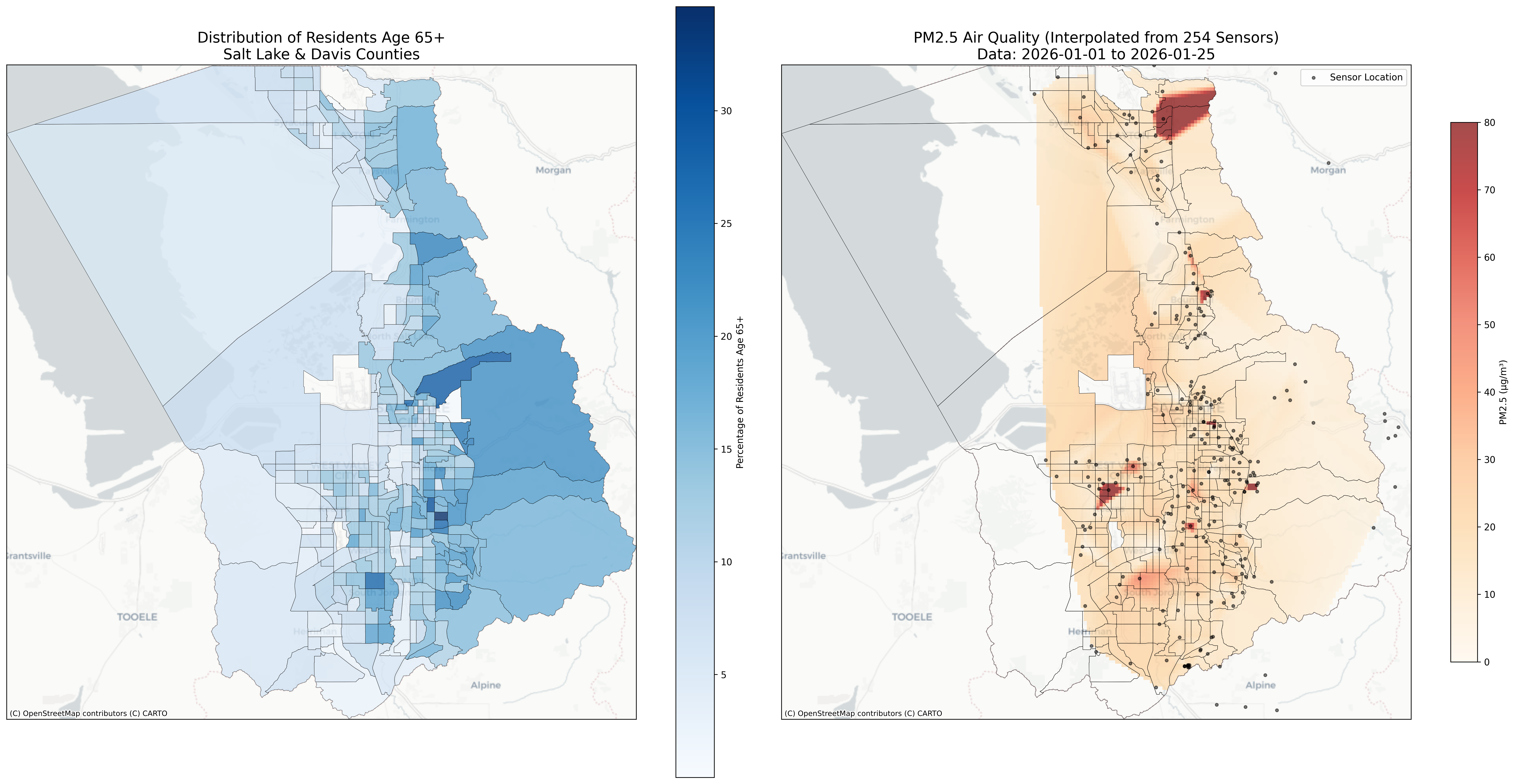
Population Age 65+ Map

Population Age 85+ Map

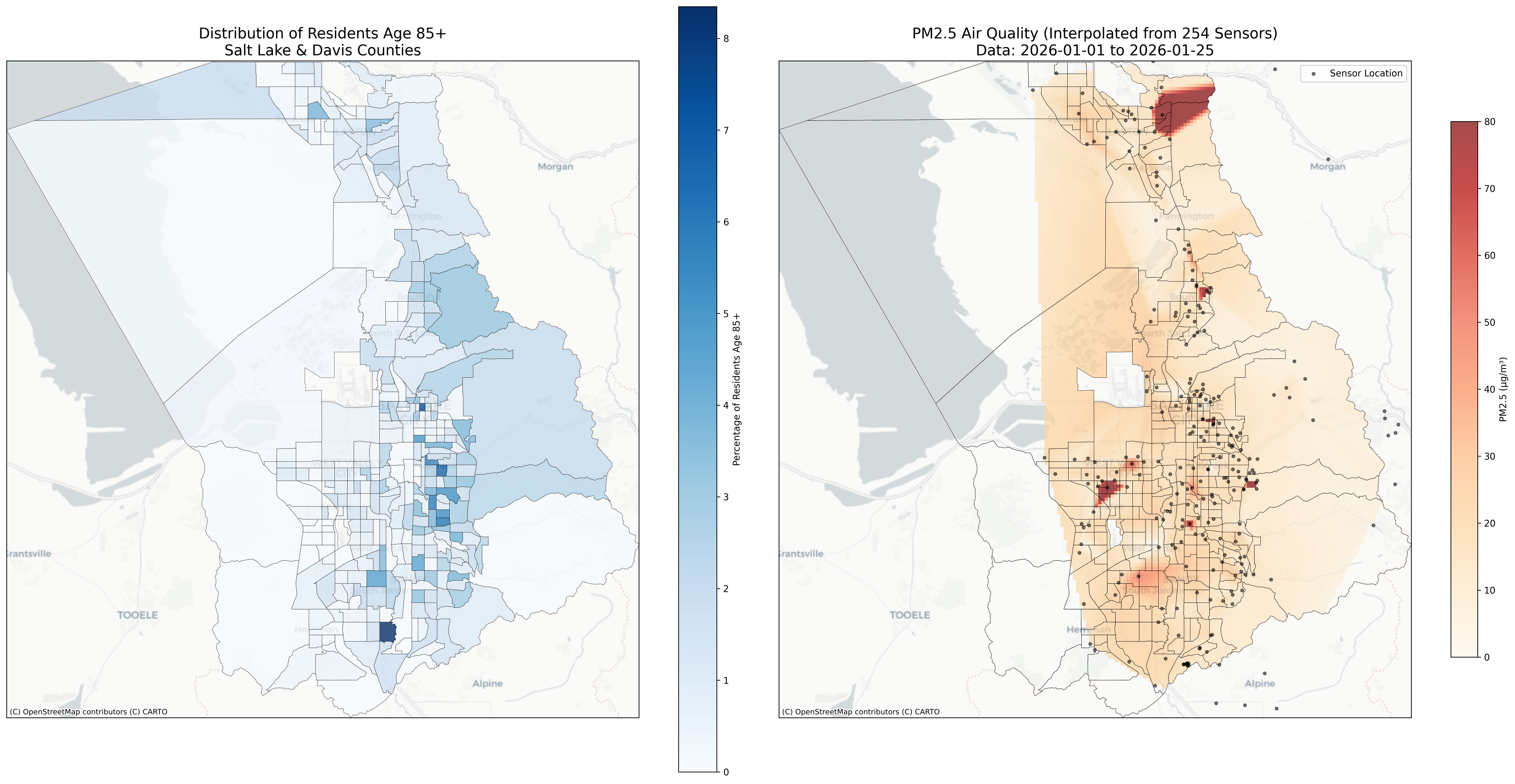
Layout (for each age group):

1. Left Panel: Choropleth map of Population Density
   • Colormap: Blues (light = low, dark = high)
   • Clearly shows concentration of seniors on East Bench and specific valley neighborhoods
   • Legend: Population percentage per census tract
2. Right Panel: PM2.5 Heatmap
   • Interpolated surface from 254 PurpleAir sensors
   • Colormap: OrRd (yellow = low, red = high)
   • Sensor locations shown as black dots for transparency
   • Spatial interpolation enables continuous surface mapping

Purpose: Demonstrate high-density sensor network capability for detailed neighborhood-level air quality visualization. Separate maps allow comparison between 65+ and 85+ population distributions and their spatial correlation with PM2.5 exposure patterns.

Data Analysis Plots

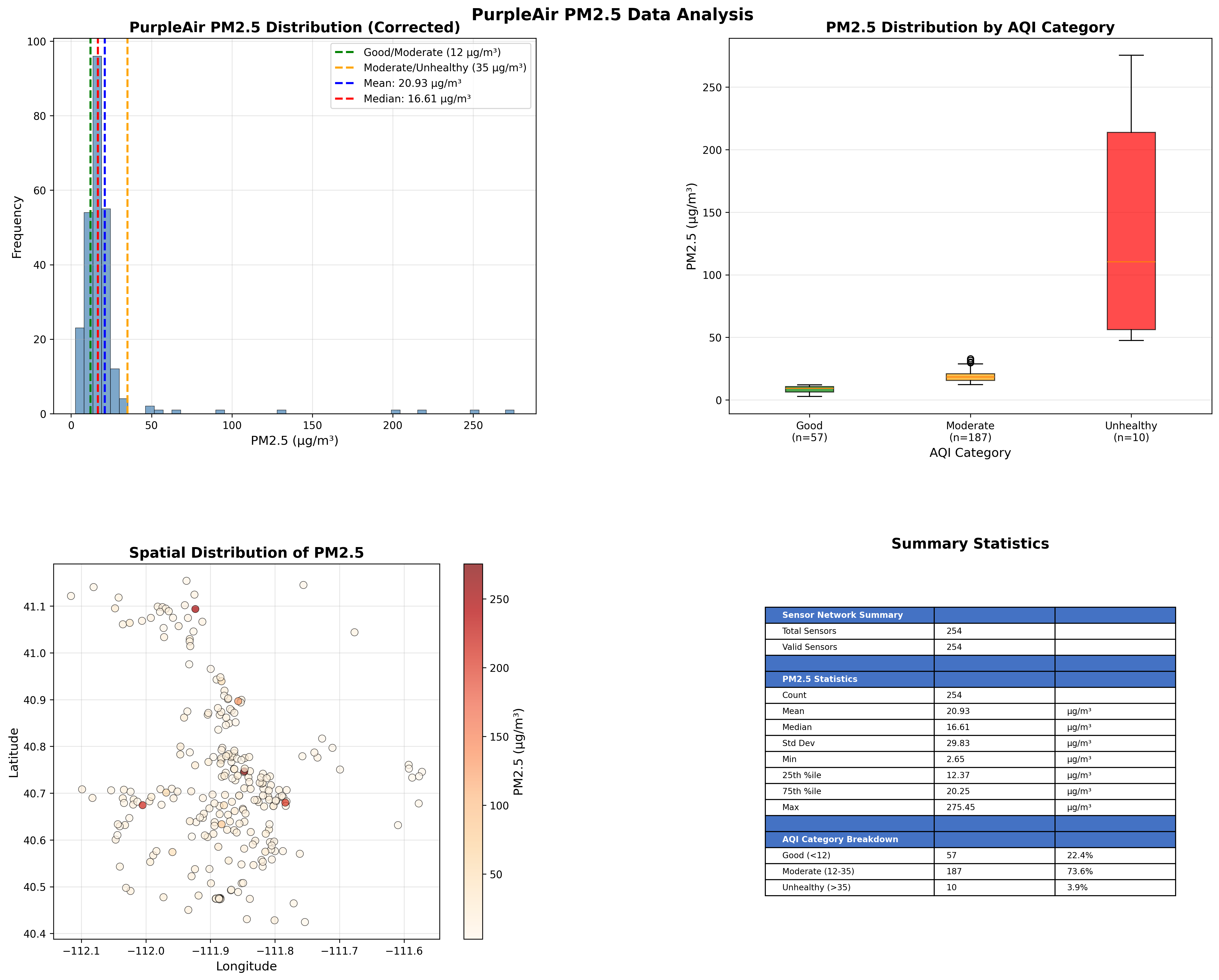
Content:

• Panel 1: PM2.5 Distribution Histogram (corrected values)
• Panel 2: Box Plot by AQI Category
• Panel 3: Spatial Distribution (Latitude vs. Longitude colored by PM2.5)
• Panel 4: Summary Statistics Table

Interactive Web Maps

Population Age 65+ Map

Interactive map - Click and drag to explore, use controls to toggle layers

Population Age 85+ Map

Interactive map - Click and drag to explore, use controls to toggle layers

• Choropleth layer for population demographics (toggleable)
• Circle markers for PurpleAir sensors (color-coded by PM2.5 level)
• Hover tooltips showing census tract information
• Clickable popups with detailed sensor information
• Layer control panel for toggling visibility
• Color-coded sensors by AQI category (Good/Moderate/Unhealthy)
• Legend with data period (January 1-25, 2026) and sensor counts
• Responsive design for desktop and mobile viewing

Key Findings

Air Quality Patterns

• Analysis Period: January 1-25, 2026
• Valid Sensors: 254 sensors with quality-controlled data
• Mean PM2.5: 20.93 µg/m³
• Median PM2.5: 16.61 µg/m³
• Range: 2.65 to 275.45 µg/m³
• Standard Deviation: 29.83 µg/m³

Air Quality Status Distribution

• Good (<12 µg/m³): 57 sensors (22.4%)
• Moderate (12-35 µg/m³): 187 sensors (73.6%)
• Unhealthy (>35 µg/m³): 10 sensors (3.9%)

Spatial Variation

• High-density sensor network reveals neighborhood-level variations
• Some areas show 2-3x PM2.5 differences between nearby neighborhoods
• Valley floor generally shows higher concentrations than bench areas
• Wide standard deviation (29.83 µg/m³) indicates significant spatial heterogeneity

Descriptive Statistics

Sensor Network Summary

• Analysis Period: January 1-25, 2026
• Total Sensor Files: 279
• Sensors in Master List: 279
• Valid Sensors Processed: 254 (after quality control)
• Sensors Filtered (Outliers >500 µg/m³): 25

PM2.5 Distribution Statistics (Corrected Values)

• Count: 254 sensors
• Mean PM2.5: 20.93 µg/m³
• Median PM2.5: 16.61 µg/m³
• Standard Deviation: 29.83 µg/m³
• Range: 2.65 to 275.45 µg/m³
• 25th Percentile: 12.37 µg/m³
• 75th Percentile: 20.25 µg/m³

AQI Category Breakdown

• Good (<12 µg/m³): 57 sensors (22.4%)
• Moderate (12-35 µg/m³): 187 sensors (73.6%)
• Unhealthy (>35 µg/m³): 10 sensors (3.9%)

Spatial Distribution

• Latitude Range: 40.4245° to 41.1540°
• Longitude Range: -112.1160° to -111.5722°

Observations:

• The wide standard deviation (29.83 µg/m³) indicates significant spatial heterogeneity in PM2.5 concentrations across the study area
• High spatial density enables capture of neighborhood-level variations not possible with sparse regulatory network
• Some sensors located in microenvironments with elevated concentrations contribute to the wide range

Data Quality Metrics

• Data Completeness: 91.0% (254 of 279 sensors with valid data)
• Outlier Filtering: 25 sensors (9.0%) filtered due to values >500 µg/m³
• Correction Applied: University of Utah Winter Inversion formula applied to all sensors
• Spatial Coverage: Dense urban coverage with sensors distributed across residential, commercial, and institutional locations
• Temporal Resolution: 60-minute averages (hourly data)